3Methodology

Author: Leonardo Pinero-Perez
Written: 2018 · Thesis, University of Texas at Arlington
Original: Full thesis · 105 pages
Contents: Chapter 1 · 2 · 3 · 4 · 5 · Appendix A: Nomenclature · References · Acknowledgments and Biographical Information

Converted from the original PDF on 8 Nov 2026 with Claude Opus 5.5. The wording is unchanged, except: my name is spelled without accents, and Tables 1.1 and 1.2, pictures in the PDF, are typed out. Equations, figures and numbering follow the original. Conversion not yet checked against the PDF.

3.1Geometry Definition

3.1.1Parameters Chosen

With the three classes of vehicles studied in the previous chapter (capsule, wing-body, and blended-body), the geometric parameters are chosen by common attributes which can be scaled in a continuum. In this way the same aspects of two radically different vehicles can be numerically compared. Additionally, these parameters must have first-order relevance to the performance of the spacecraft. For instance, it would not make sense to include the dimensions of a crew entry hatch as these would have a negligible effect on vehicle parameters such as volume available, structural weight, or lift-to-drag ratio. It is important to state this now, as one of the largest differences between many of the representations of vehicles studied here and their real-world analogues is that their windshields disrupt a simpler design. Obviously, there was a second-order correction for pragmatic reasons, specifically pilot visibility (even if that means deviating from the conceptual aerodynamic design).

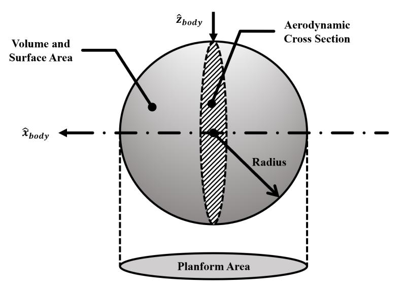
Three outlines in a row, joined by arrows: a winged spaceplane like the Space Shuttle, a lifting body, and a delta-winged shape. — Figure 3.1Different Historical Configurations must be able to Relate on a Continuum

The first parameter is chosen for its simplicity in fully describing a body with one radial dimension: a sphere. Already, this shape has characteristics that could be assessed in terms of re-entry performance (volume, planform area vs. surface area, structural weight, etc.). This simple configuration is shown in Figure 3.2, using aircraft coordinates along with first-order variables to be used in defining vehicle performance.

Shaded sphere on a body x axis, labelled with its radius, its volume and surface area, the aerodynamic cross section through it, and its planform area below. — Figure 3.2Spherical Spacecraft Design as a Re-entry Aircraft

The sphere, however, is not used because it is not an advantageous configuration given the physics of aerodynamic flight. However, if one sufficiently alters the environment or mission, the sphere can quickly become more attractive. This is exemplified in the Apollo program, where the shape of the lunar lander ascent stage was never designed to interact with the atmosphere, so structural weight became the largest concern and a spherical shape was chosen. If we were to create an environmental continuum between that of Earth sea-level atmosphere and a vacuum (described by density and atmospheric scale height), one could also assess the performance of different shapes according to some parameter which increases slenderness.

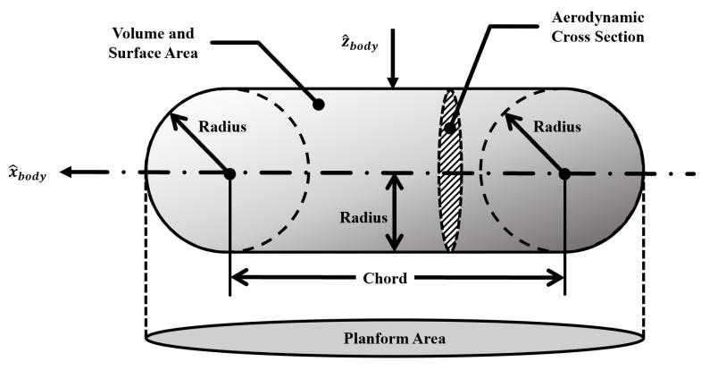
This parameter is the chord length of what used to be a sphere (which only had a radial parameter). This new parameter duplicates the sphere and specifies the distances between the two bodies. The entire geometry is still closed by a geometric loft, as shown in Figure 3.3. An important aspect of this choice is that a single sphere (as shown in Figure 3.2) can still be created by setting the chord length to approach zero. These two parameters defined by these rules can build pill shapes and can already approximate the fuselage of atmospheric aircraft.

Capsule-shaped body of two hemispheres joined by a cylinder, labelled with the radius, the chord between the hemispheres’ centres, volume and surface area, aerodynamic cross section and planform area. — Figure 3.3New Generalized Design Now defined by Chord and Radius

It is evident that the most common aspect of all space vehicles is that they have a body which could store fuel, propulsion, and payload required to complete a mission. The overall shape chosen is a rounded cross section, which can approximate other polygonal cross sections such as a diamond or trapezoid. The selection of a rounded cross-section also accurately represents fuselage bodies and axially symmetric capsules.

Two more parameters are added to allow for design flexibility. The first added parameter is simply adding a degree of freedom to the pill design: the radii of the pill-shape can now have different values. By doing this, conical shapes can be approximated, and the nose radius can be decreased while allowing a large aft radius for storing fuel and a propulsion system in the aft region.

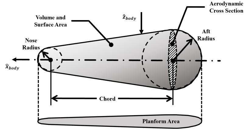
Tapered body with a small spherical nose and a larger rounded aft end, labelled with the nose radius, aft radius, chord, aerodynamic cross section, volume and surface area, and planform area. — Figure 3.4Generalized Design after Unlocking the Equal Radii Constraint

At this point, some new rules are given to this general design. The aft radius will now only be used to describe the aft cross section, which makes this dimension constrained to the y-z plane in the aircraft body coordinates. This is due to the impracticality of a rounded or domed aft section configuration, as this area is usually flat to be a flush mate with lower stages, reducing the structural weight of the combined vehicle. This is actually one of the disadvantages of using an ovoid shape for a re-entry capsule, as a truss system must be added to the combined vehicle for proper interface with lower stages [12]. This truss system will most likely require aerodynamic fairings to endure the atmospheric loads during launch. Additionally, this staging interface can be reserved for an area to place the nozzle of the propulsion system.

The second parameter added is the span, converting the axially-symmetric cross-section to an elliptical one. This further constrains the aft radial parameter to one dimension along the z-axis and the nose radius to the x-z plane. By doing this, the cross section can be changed to more accurately describe blended body vehicles. As will be later discussed, increasing the span increases the planform area and the surface area. These new geometric conditions finalize the body section of this generalized design.

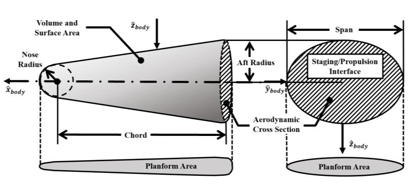
Side and end views of the generalized body: a tapered body with its nose radius, aft radius and chord, and an elliptical aft cross section whose width is the span, marked as the staging and propulsion interface. — Figure 3.5General Design Described by Nose and Aft Radii, Chord, and Span

It is important to re-iterate that these four parameters can be made into special cases such as the pill shape or sphere by setting the span to equal the radii, set the radii equal to each other, and possible setting the chord to zero (if a sphere is desired). The main idea is that the original, simple geometry is not lost, but flexibility and applicability is increased by adding these four important parameters.

3.1.2Superimposed Wing

The body of the spacecraft is now constructed, and this alone can describe many re-entry vehicles, such as capsules or lifting bodies. Again, since there are only four geometric parameters, second-order characteristics such as windshields or multiple sweeps cannot be described. However, first-order trends can be identified along parameter axes for these vehicles. This theme continues by adding a second element to capture a major configuration feature of historical re-entry vehicles: the wing. Vehicles such as the Dyna Soar or the X-37 cannot be described only defining a fuselage, so the option to superimpose a wing body must now be included.

The existing fuselage is now rotated to be facing the x-y plane, demonstrating the planform area of the vehicle. The key parameter affected by adding a wing is the planform area with a negligible increase in volume. The increased surface area with minimal wing volume creates a radically increased structural weight, which must include thermal protection. Minimal wing volume also does not allow the storage of fuel or payload. This is the cost of increasing the planform area.

The wing is defined by two new geometric parameters: the wing’s root chord and the wing span. The end-points of these dimensions create a delta-shape, which is the simplest to define and characteristic of planforms in the hypersonic speed regime.

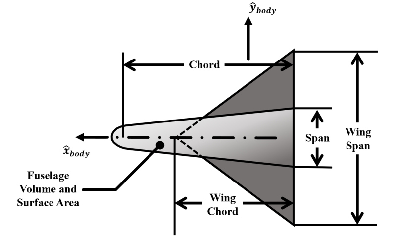
Planform of a slender fuselage with a dark delta wing superimposed at its rear, labelled with chord, span, wing chord and wing span along the x and y body axes. — Figure 3.6Generalized Fuselage with a Superimposed Generalized Delta Wing

The addition of a wing can be further defined by a dihedral angle for directional stability. However, to do this the x-y plane projection (planform area) is decreased without changing the overall surface area associated with zero volume (wing size). Directional stability is obtained by incurring a structural weight cost if the lifting planform area is held constant.

3.1.3Historical Validation of Geometry

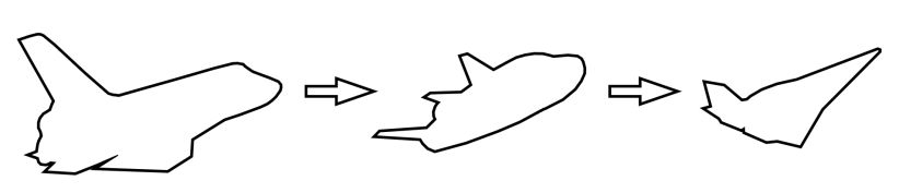
With these parameters, a first-order configuration can now be made to represent the majority of historical vehicles. The sample of historical vehicles is now shown in this section to validate the geometric definitions built in this section.

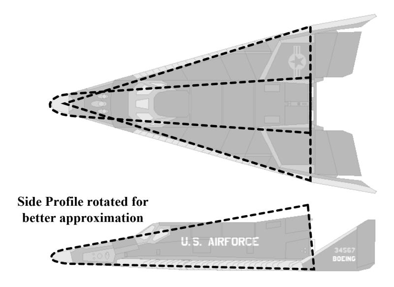
Figure 3.7X-20 Dyna Soar Represented by Geometric Parameters [18]

There is some obvious error (notice the windshield), but as mentioned before, this an acceptable loss in order to build a parametric continuum between this configuration and something like a Mercury capsule, as shown in Figure 3.8.

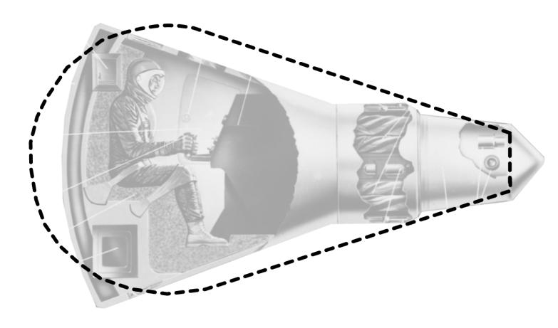
Cutaway of the Mercury capsule with an astronaut seated inside, overlaid by a dashed outline of the parametric shape: a large blunt aft end tapering to a small nose. — Figure 3.8Mercury Capsule Represented by Geometric Parameters *[19]*

The nose radius is now shown to be larger than the aft radius, but it still remains the nose radius as its definition extends along the x-z plane as opposed to being constrained to the z-axis like the aft radius. It is also worth noting that unlike the X-20 Dyna Soar, the Mercury capsule is axially symmetric, so its span parameter is set to be equal to the aft radius. The parameters are set so that there is a close approximation for volume and surface area. However, to do this, the nose radius is decreased, which will over-estimate the heating loads. There are also no wings superimposed on this vehicle.

Lastly, the geometric parameters will represent the focus vehicle of the author’s senior project, shown in Figure 3.9. This vehicle is a blended body with a trapezoidal cross section (approximated here as an ellipse scaled to equal cross-sectional area). Without wings, this lifting body has a high slenderness and is expected to be the highest performing vehicle.

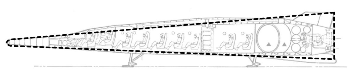
Side-view drawing of the Model 176 with its seated passengers, overlaid by a dashed outline of a slender tapered body. — Figure 3.9Model 176 Represented by Geometric Parameters *[8]*

It has been shown that the parameters presented can re-create a wide variety of historical spacecraft upper stages. The next stage is to take these parameters and link them to performance measures which can assess the viability of these configurations across several missions and environments.

3.2Geometry Analysis

3.2.1Planform Area

The fuselage planform area is easily computed as a function of the geometric parameters, which are now abbreviated as proper variables: $r_{a f t}, c, r_{n o s e}, b$ . The nose’s contribution is first ignored and can be computed as a half-ellipse. As seen by the Mercury capsule, the nose planform area can make up a significant portion of the total planform area.

S_{b o d y} = S_{l o f t} + S_{n o s e} = [\frac{b c}{2} (1 + \frac{r_{n o s e}}{r_{a f t}})] + [\frac{π b r_{n o s e}^{2}}{4 r_{a f t}}]

If a wing is added, the shared planform area between the two bodies (wing and fuselage) is not computed to avoid double-counting. Instead, only the exposed planform area is computed.

S_{w i n g} = \frac{\frac{1}{2} {(b_{w i n g} - b)}^{2}}{\frac{b}{c} (1 - \frac{r_{n o s e}}{r_{a f t}}) - \frac{b_{w i n g}}{c_{w i n g}}}

Sometimes, the wing geometry may be modified to a point where it is completely enveloping the body, in which case the planform area of the vehicle is equal to the planform area of the wing. Conversely, the wing may become completely obscured by the body and output a negative value by mathematical definition, in which case the planform area due to the wing is told to become a value close to zero.

3.2.2Wetted Area

Wetted area is computed by numerically computed by taking the circumference of the ellipse and extruding it by a small step size along the x-axis. This step size is set as a small proportion of chord length. It is important to note that the numerical error increases as the sweep angle decreases, as each step along the x-axis has a 90-degree sweep. Since hypersonic vehicles typically have a high sweep angle, small-angle assumptions will hold true for each step along the x-axis.

There is no exact solution for finding the circumference of an ellipse, so this is also an approximation and surprisingly complicated [20].

C i r c (x) \approx f (r (x), \frac{b (x)}{2}) = f (p, q)

= π (p + q) (\frac{3 (p - q)^{2}}{(p + q)^{2} (\sqrt{- \frac{3 (p - q)^{2}}{(p + q)^{2}} + 4} + 10)} + 1)

Where the local variables are found as a function of geometric parameters and axial location:

r (x) = r_{a f t} + \frac{r_{n o s e} - r_{a f t}}{c} x

b (x) = \frac{r (x) b}{r_{a f t}}

The staging/propulsion interface in the aft part of the vehicle is not considered for wetted area, as it is not exposed to re-entry conditions. In some special circumstance, considering this interface area as wetted area is as easy as adding the area of that ellipse.

The nose surface area is that of a half ellipsoid, which is also a complicated mathematical approximation [20].

S_{w e t} = (S_{w e t})_{l o f t} + (S_{w e t})_{n o s e} = [\int_{0}^{c} C i r c (x) H d x] + 2 π {[\frac{1}{3} (2 {(\frac{r_{n o s e}^{2} b}{r_{a f t}})}^{1.6} + r_{n o s e}^{3.2})]}^{\frac{1}{1.6}}

Where $H$ is user-determined as a trade-off between accuracy and computational speed. In this study, it is set to one two-hundredth of the chord length as this calculation will be made many thousands of times each time the script is run.

3.2.3Volume

Volume is computed similarly to wetted area, where the lofted section is computed numerically along x-axis steps sized as a small proportion of the vehicle chord. Instead of local circumference, local area is computed. The formula for local elliptical cross-sectional area is simpler and exact, using the local variables $r (x)$ and $b (x)$ .

A (x) = f (r (x), \frac{b (x)}{2}) = f (p, q) = π p q

The lofted volume is found by combining the numerically integrated lofted volume and the nose volume (half-ellipsoid). The wing does not contribute to the total vehicle volume.

V O L = V O L_{b o d y} = V O L_{l o f t} + V O L_{n o s e} = [\int_{0}^{c} A (x) H d x] + [\frac{2 π r_{n o s e}^{3} b}{3 r_{a f t}}]

3.2.4Küchemann’s Tau

Tau is simple to calculate, as it is a ratio function of two previously computed variables: volume and planform area. Tau is important for determining the aerodynamic characteristics of the vehicle, particularly lift-to-drag ratio. It is defined by this ratio [7].

τ = \frac{V O L}{S_{p l a n}^{1.5}}

3.3Vehicle Analysis

3.3.1Structural Weight

The structural weight is considered to be linearly correlated to the wetted area according to a technology index. This index is specific to the state-of-the-art in materials science, whose value is found in literature for re-entry vehicles. It is worth noting that the smaller nose radii will disproportionately require a higher structural weight due to an increased heat flux.

W_{s t r} = I_{s t r} S_{w e t}

The structural index is set to $I_{s t r} = 17.1 \frac{k g}{m^{2}}$ for re-entry vehicles [7].

3.3.2Propulsion System

The propulsion system is included according to typical orbital maneuvering engines considered sufficient to follow the proposed re-entry and synergetic trajectories. The propulsion system is paid for by engine weight and volume, and in return will give the vehicle a property of non-zero specific impulse, depending on the type of engine “bought” by the weight and volume budget.

The payload weight and volume will now affect the remaining volume available for propellant. A vehicle with maneuvering capability must have enough volume available to contain the engine and payload. In this way, there is volume available for propellant.

V O L_{p p l} = V O L - V O L_{e n g} - V O L_{p a y}

Where the following condition must be met for a maneuvering vehicle:

V O L > V O L_{e n g} + V O L_{p a y}

Conical body outline holding a dashed payload volume near the nose and a dashed engine volume at the aft end; the remaining space is labelled usable volume. — Figure 3.10Volume Breakdown for First-Order Vehicle

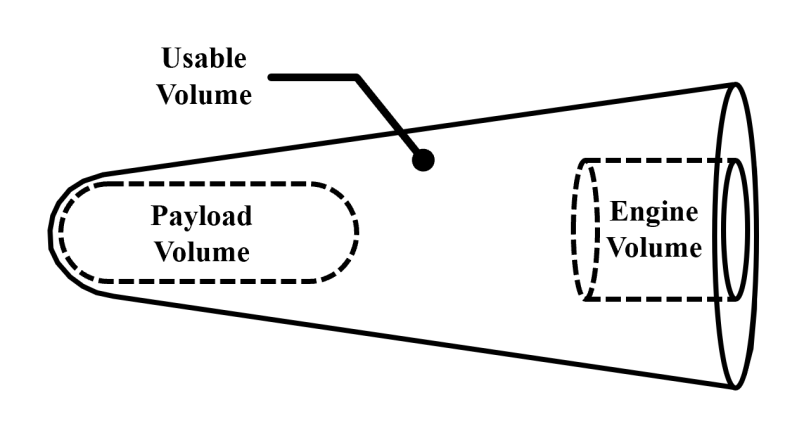
The rest of the volume will be filled with propellant, where the volume of the structure is considered to be negligible for first-order analysis. The weight of the propellant is determined by the mixture ratio required by the engine.

3.3.3Delta V

The weight of the propellant and the structural weight will determine the vehicle’s mass ratio.

M R = \frac{W_{f u l l}}{W_{e m p t y}} = \frac{W_{e n g} + W_{p a y} + W_{s t r} + W_{p p l}}{W_{e n g} + W_{p a y} + W_{s t r}}

This mass ratio combined with the specific impulse will determine the delta V available to the spacecraft by the rocket equation.

Δ V_{a v a i l a b l e} = g_{\oplus} I_{s p} \ln (M R)

3.3.4Lift to Drag Ratio

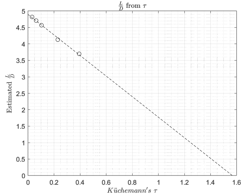
The lift-to-drag ratio can be computed as an empirical function of tau. This is found in literature from the result of flight and wind tunnel testing of various bodies [21].

\frac{L}{D} = \frac{A (M + B)}{M} [\frac{1.0128 - 0.2797 \ln (\frac{τ}{0.03})}{1 - \frac{M^{2}}{673}}] where A = 6 and B = 2

This equation applies only to a specific range of tau, so conditional statements are created to bound the possible lift-to-drag ratios between zero (ballistic) and three (highest expected performance).

A modified estimation for lift-to-drag performance is created from data points found in reference [22]. The trend is strongly correlating to a negative linear slope as shown in Figure 3.11.

Plot titled “L/D from τ” of estimated L/D against Küchemann’s τ from 0 to 1.6: a few circled data points between about 4.8 and 3.7 at low τ, and a dashed line falling straight from about 4.9 to zero near τ = 1.55. — Figure 3.11Alternative Lift-to-Drag Ratio Estimation Method from Tau

3.4Performance Analysis

3.4.1Payload Capability

The first assessment of performance is that of the payload capacity of the vehicle with respect to the launch weight. The full weight of this upper-stage vehicle is the payload of the lower stages. According to the rocket equation, increasing the full weight will significantly increase the weight of the launch vehicle. This will increase the total cost of carrying a given payload. The user will specify the importance (signified as $A_{P I}$ ) of payload capability depending on the anticipated budget for the launch vehicle.

P I_{p a y} = \frac{A_{P I} W_{p a y}}{W_{e n g} + W_{p a y} + W_{s t r} + W_{p p l}}

Vehicles which place high priority on $P I_{p a y}$ will be driven to reduce the propellant and structural weight by decreasing the geometric dimensions. Consequentially, increasing the importance of this performance index will take a toll on the other two performance indices.

3.4.2Synergetic Maneuver

The vehicle’s ability to perform a synergetic inclination change is a function of the available fuel and aerodynamic properties. This assessment is determined from Nyland’s analysis of synergetic maneuvering according to $Δ V_{a v a i l a b l e}$ and $L / D$ .

The vehicle’s capability is assumed to be at a maximum performance when the angular change of inclination reaches 90 degrees. This is due to the assumed conical angle of 45 degrees, the value of which was selected as the best compromise to minimize maneuver heating and achieve a full inclination maneuver [5].

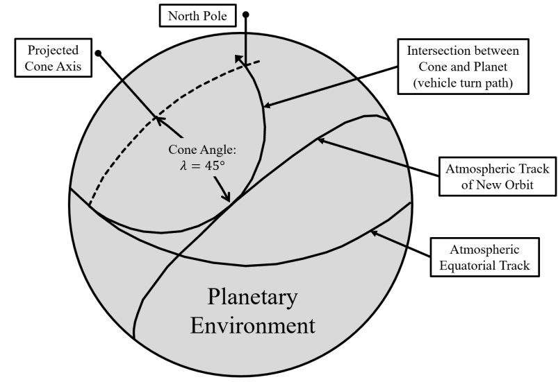
Sphere labelled Planetary Environment, showing the north pole, the projected cone axis, a cone angle λ = 45°, the intersection between cone and planet (the vehicle’s turn path), the atmospheric track of the new orbit, and the atmospheric equatorial track. — Figure 3.12Synergetic Maneuver for a 45-degree Turn-Cone Angle

If the craft continues past this inclination change of 90 degrees, the new orbital inclination will lower, but in the opposite direction. For the purposes of the proposed missions, the author has reasoned that changing the orbital direction is not useful, as this can be decided by the starting conditions before the parking orbit. For these reasons, the maximum inclination for any craft will be 90 degrees. Any further geometric improvements towards increasing performance will garner no additional value to the performance index.

The user will now specify the importance of an inclination change. This can be important for a surprise reconnaissance mission as mentioned in the introduction. Additionally, the author will propose a mission to change inclination to rendezvous with an orbital station at a set inclination on another planet. Due to an initial inclination advantageous to a transfer orbit between the Earth and this planet, an inclination change would be required in orbit. This mission may limit the payload capability due to a necessary aerodynamic performance. In fact, higher aerodynamic performance may aid in reducing the required fuel to make the inclination change. Regardless, the performance of the synergetic maneuver is determined as follows, according to a user-specified weighting factor.

P I_{i n c} = B_{P I} \frac{2 (Δ i)}{π}

Like the previous performance index, the performance variable $Δ i$ is normalized by the maximum value in radians. For a desired inclination, the $B_{P I}$ must be set such that costs increase as a function of the maximum value. A good starting approximation for the weight can be defined by the desired inclination.

B_{P I} \approx \frac{π}{2 (Δ i)_{d e s i r e d}}

The inclination change of a particular design is assessed according to $Δ V_{a v a i l a b l e}$ and $L / D$ . A proportion of the propellant is used to initiate descent for both one maneuver and the final descent, so multiple synergetic maneuvers incur that initial impulse cost.

The total inclination change is based on the turn angle achieved along the cone-sphere intersection circle with a cone angle of $λ = 45 °$ . The further the craft travels along this angle, the more velocity lost due to drag along this atmospheric circle. This velocity loss is determined by the range function denoted as $F (\bar{u}, λ)$ . The full analysis, made by F. S. Nyland of the Rand Corporation, is found in reference [5].

The turn angle achieved is determined by tolerable velocity loss and the aerodynamic performance of the craft.

φ = \frac{1}{2} \frac{L}{D} [\ln | F ({\bar{u}}_{i}) | - \ln | F (\bar{u}) |]

The range function based on velocity change is shown below.

F (\bar{u}, λ) = 1 - \frac{{\bar{u}}^{2}}{(\sin λ)^{2}} - \frac{1}{\sin λ} \sqrt{\frac{{\bar{u}}^{4}}{(\sin λ)^{2}} - 2 {\bar{u}}^{2} + 1}

From these equations, the inclination change can be determined from the intersection cone and the turn angle achieved for each spacecraft.

Δ i = \sin^{- 1} [\sin φ \cos λ \sqrt{1 + \frac{1 - \cos φ}{1 + \cos φ} (\sin λ)^{2}}]

This analysis is implemented into the methodology and plotted for Earth values.

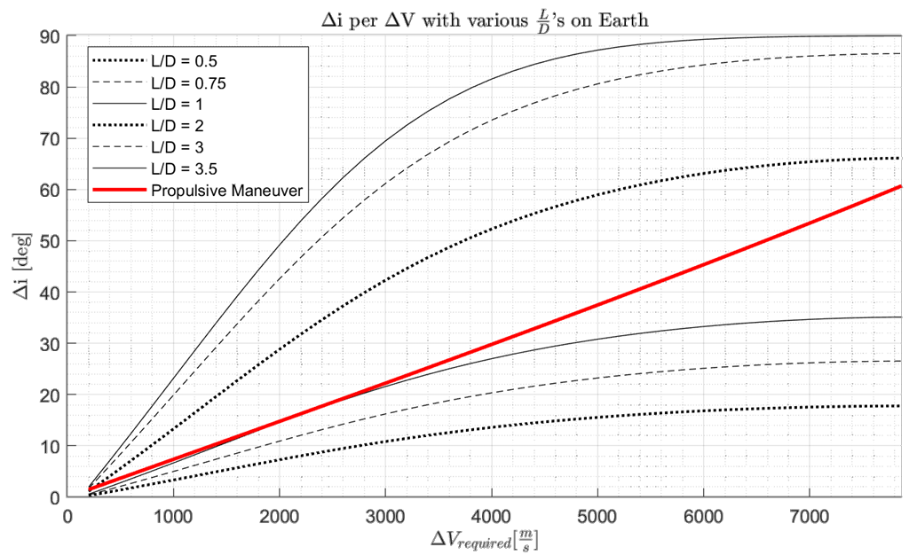
Plot titled “Δi per ΔV with various L/D’s on Earth”: inclination change in degrees against required ΔV in m/s up to about 7,900, one curve each for L/D from 0.5 to 3.5 and a straight red line for a propulsive maneuver; the higher the L/D, the faster the curve rises toward 90 degrees. — Figure 3.13Lift-to-Drag Ratio Effect on Expended $Δ V$ for an Earth Inclination Change

The code has been generalized to be applicable to any atmosphere with sufficient density. It is important to note that atmospheric models which are significantly less dense than that of Earth will compute an initiated turn below the planet’s surface. However, even the atmosphere of Mars has an equivalent atmospheric density above its surface as the density used in Nyland’s analysis.

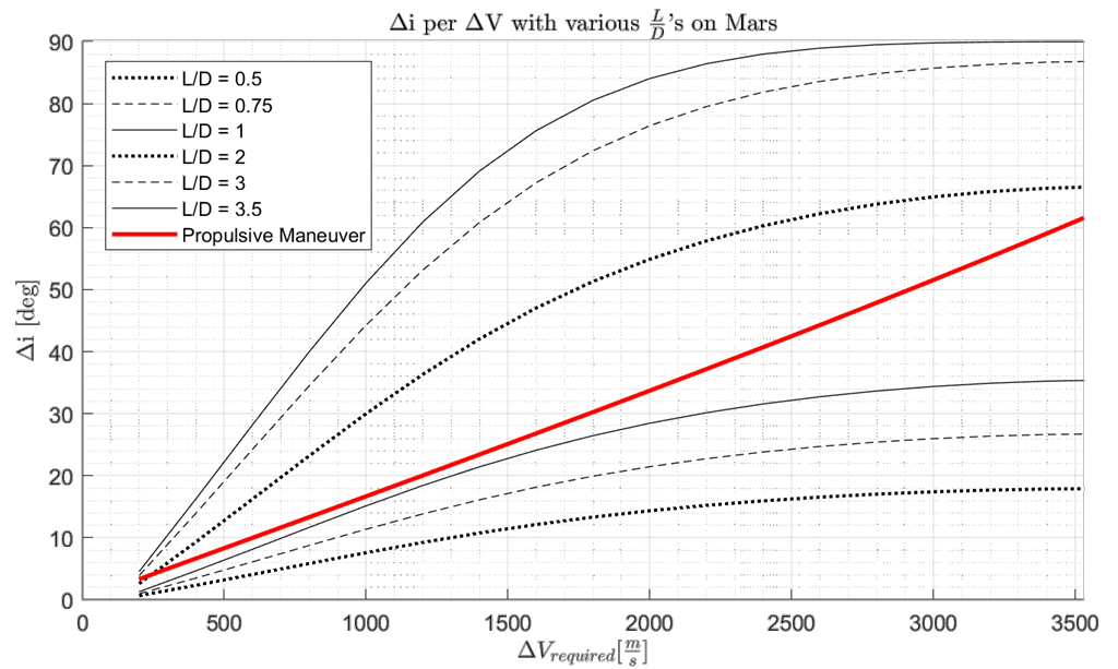
Plot titled “Δi per ΔV with various L/D’s on Mars”: the same curves for Mars, against required ΔV up to about 3,500 m/s. — Figure 3.14Synergetic Maneuvering Requirements on Mars

The requirements on a spacecraft orbiting 200 km above the Martian surface are significantly less than those required of initiating from a 200 km Earth orbit, but the comparison between a synergetic maneuver and a propulsive maneuver remains the same. It seems as though the inclination change requirements scale similarly with the planetary body (though not exactly the same, as variations between atmospheric heights require different periapsis altitudes for descent). In the Martian atmosphere, the turn is initiated at around 37 km above the surface, which is comparable to a turn initiation at about 64 km above sea level on Earth.

3.4.3Descent Trajectory

The descent performance is assessed by three components, each with their own user-specified weights: cross-range, load factor, and heating. This is the only performance index component which itself contains multiple components. The effect of this is that these sub-components are less important if the performance index weights are equal. For this reason, if the mission calls for a descent component to be held at the equivalent value of a higher-level component such as inclination change, the performance weights must compensate for this. This hierarchy is more clearly demonstrated in the next subsection.

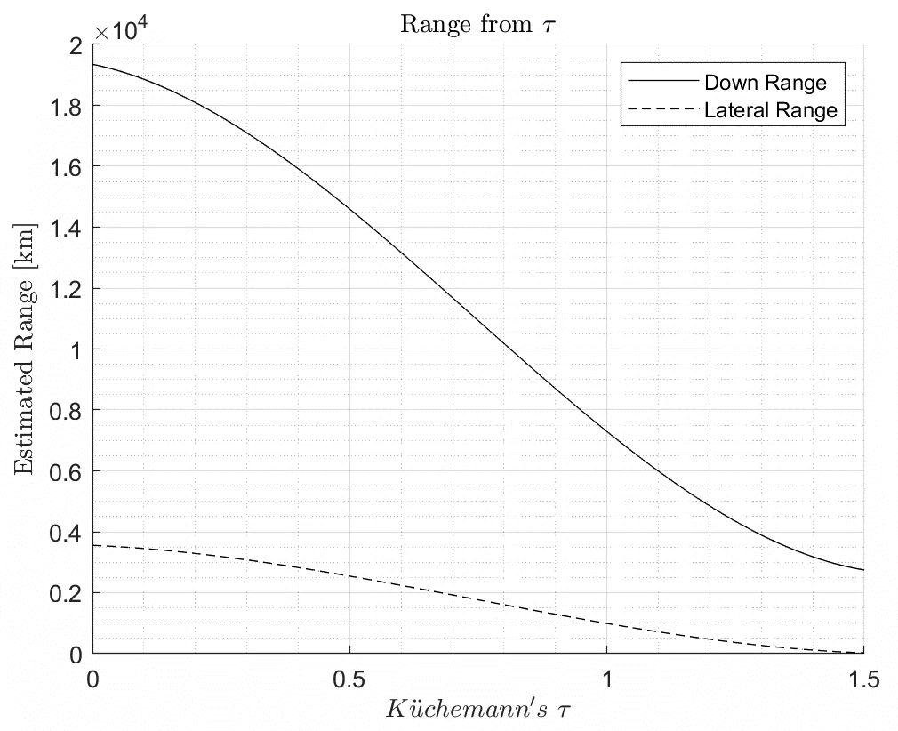
P I_{d e s} = C_{P I} \sqrt{\frac{{(A_{d e s} \frac{s}{2 π R_{0}})}^{2} + {(B_{d e s} | 1 - \frac{a_{l o a d}}{10 g_{0}} |)}^{2} + {(C_{d e s} | 1 - \frac{\dot{q}}{{\dot{q}}_{m a x}} |)}^{2}}{A_{d e s}^{2} + B_{d e s}^{2} + C_{d e s}^{2}}}

The cross-range of a spacecraft can be estimated by the lift-to-drag ratio and is later normalized by the planet’s circumference. While a quick historical estimate is used below [7], the analysis found in reference [3] can provide more accurate and generalized cross-range analysis.

Lateral Range [km] = L R

= 0.539957 [1.667 + 68.016 (\frac{L}{D}) + 706.67 {(\frac{L}{D})}^{2} - 91.111 {(\frac{L}{D})}^{3}]

Down Range [km] = D R = 0.539957 * 4866.6 + 4.70417 (L R)

The range is plotted as a function of tau in Figure 3.15 as lift-to-drag can be estimated by this geometric parameter.

Plot titled “Range from τ” of estimated range in km (×10^4) against Küchemann’s τ from 0 to 1.5: down range falls from about 19,000 km to about 2,800 km, and lateral range from about 3,500 km to near zero. — Figure 3.15Vehicle Descent Range as a Function of Tau

The aerodynamic acceleration loading is dependent on the aircraft’s basic aerodynamic characteristics and its current flight condition.

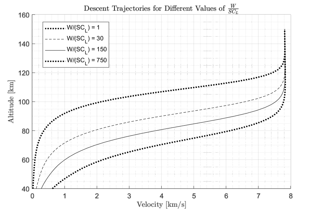
Plot titled “Descent Trajectories for Different Values of W/SC_L”: altitude in km against velocity in km/s, one glide curve each for W/(SC_L) = 1, 30, 150 and 750; all descend from about 150 km at about 7.8 km/s, and the lower the value, the higher the glide. — Figure 3.16Steady Glides for Differing Vehicle Parameters

This flight condition is dependent on the point along a pre-determined steady glide as shown in Figure 3.16.

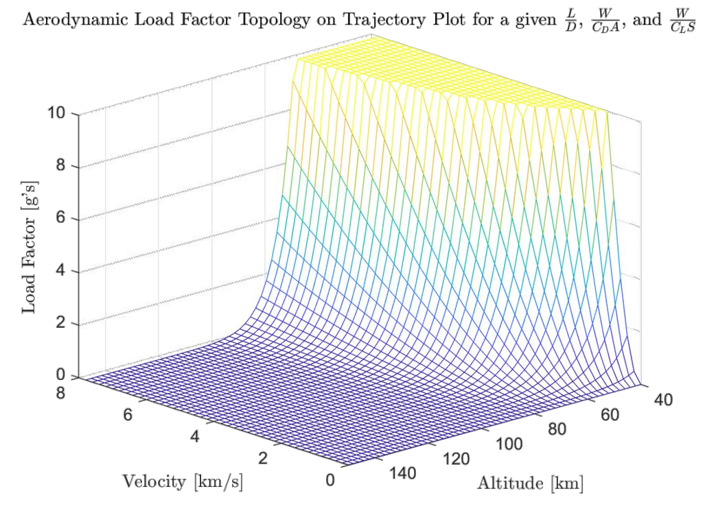
Surface plot titled “Aerodynamic Load Factor Topology on Trajectory Plot for a given L/D, W/(C_D A), and W/(C_L S)”: load factor in g against velocity from 0 to 8 km/s and altitude from 40 to 140 km; it stays near zero over most of the range and climbs steeply to about 10 at high velocity and low altitude. — Figure 3.17Aerodynamic Load Factor with Fixed Vehicle Parameters

Determining the maximum heating rate involves the same inputs as acceleration loading with the nose radius. This performance parameter is unique in that it is directly dependent on this one geometric parameter.

3.4.4Total Performance

The vehicle must be assessed by a single parameter according to the weights selected by the user. These are normalized according to their maximum values.

P I_{t o t} = \sqrt{\frac{{(P I_{p a y})}^{2} + (P I_{i n c})^{2} + (P I_{d e s})^{2}}{A_{P I}^{2} + B_{P I}^{2} + C_{P I}^{2}}}

In summary, these performance indices are valued according to user preference in two hierarchy levels. This hierarchy is demonstrated with its associated user-specified weight in Figure 3.18.

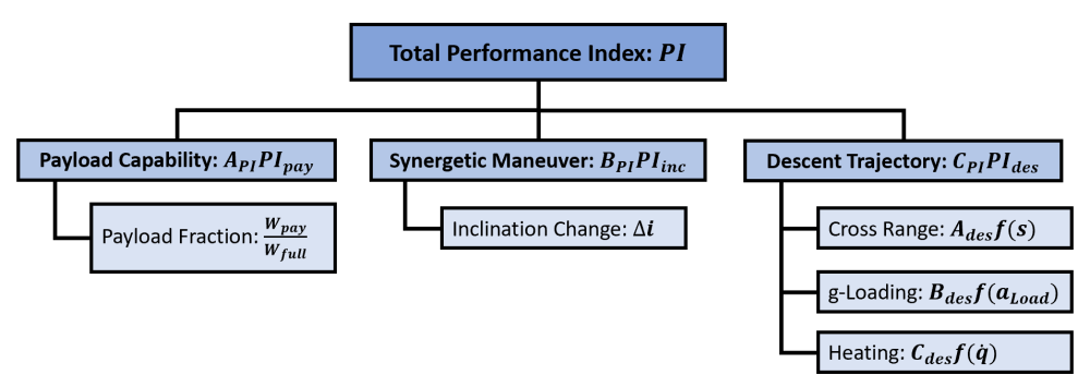
Tree diagram: the total performance index PI splits into payload capability (A_PI PI_pay, from the payload fraction W_pay/W_full), synergetic maneuver (B_PI PI_inc, from the inclination change Δi) and descent trajectory (C_PI PI_des, from cross range, g-loading and heating). — Figure 3.18User-specified Weights define Mission Priorities

From here, the total performance index of any combination of the geometric parameters can be determined. By tweaking a geometric parameter, the user can view how this changes the performance. By this method an optimization routine can be applied to the methodology to see how a design can evolve to meet the mission requirements.

Spotted an error, or want to reply? Email me: leonardo.pinero42 [at] gmail [dot] com