VIIISynthesis
- Author
- Leonardo Pinero-Perez
- Written
- 2018 · Report, University of Texas at Arlington
- Original
- Full report · 120 pages
- Contents
- Nomenclature · Chapter I · II · III · IV · V · VI · VII · VIII · IX · X · XI · Appendix · References
- Ref
- MAE 4351-2018
Converted from the original PDF on with Claude Opus 5.5. The wording is unchanged, except: two classmates’ names are replaced by their roles, Figure 54 (an attendance sheet) is omitted, and my name is spelled without accents. Equations, figures and numbering follow the original. Conversion not yet checked against the PDF.
ASizing
The sizing method used is dependent on the industry capability index (ICI), which is constructed by structural weight, mission requirements, and slenderness. Payload and fuel volume fractions available are also drivers of sizing. This index will size the planform area of the vehicle according to mission requirements.
The ICI is a measure of available technology and is defined such that performance can increase with increasing structural or propulsion capabilities [2]. This is very useful for sizing high-performance aircraft where failure of a concept is often due to a lack of available technology, as it was for many spaceplane concepts after the Apollo program [1]. As shown in the MDA, sizing begins with an understanding of the mission requirements, and technological capability will be built off of 176 data. The ICI is calculated as follows:
Propulsive Index:
Structural Index:
Industrial Capability Index (ICI):
To obtain a starting value, the values for the Model-176 are used in this equation, provided by the disciplines. Other geometric values allowed the team to find sizing parameters:
We now have the ICI for the 1964 Model-176. This provides a starting point for iteration. Producing a carpet plot with variables of planform area versus industrial capacity will now prove useful. It is desirable for the hypersonic vehicle design to be as small and light as possible, since that will drive down launch costs immensely (this is an upper stage so weight reduction here greatly compounds in the rocket equation).
Sizing is conducted from the mission profiles and completed by synthesis engineer Rashi Jain. The two military variants converged to a proper planform size at the time of presentation, but the civilian variant has yet to converge. Fortunately, this variant is not design critical given its low delta-V mission profile and light payload for a geometry and volume budget equivalent to the other two military variants.
BDisciplinary MATLAB Functions
In order to condense the synthesis script, the disciplines have encapsulated their methods into MATLAB functions. Disciplines have multiple functions called, so user guides are documented in this section. This is an important high-level method which will allow the team to debug any inconsistencies within the hypersonic vehicle’s design script.
Performance Functions [15]:
Function Name: subsonic_perf.m Brief Description:
- Uses basic aero variables and atmospheric properties to calculate the range, optimum glide trajectory, and landing field characteristics for the vehicle (uses Raymer’s method, very similar to xb-70 method)
Inputs: subsonic_perf(LDmaxsub,CLsub,CLmaxsub,Ssub,Wsub,hsub);
- LDmaxsub = subsonic maximum lift drag ratio
- CLsub = CL associated with max lift-drag ratio
- CLmaxsub = overall maximum possible subsonic CL
- Ssub = reference area with straight wings deployed
- Wsub = probably vehicle empty weight
- hsub = initial altitude for flight phase
Constants:
- g = 9.81 (gravity in SI)
- atmos function
Outputs: [Range, Vapp, Sg, gammaa] , plot: altitude vs. velocity for optimum glide
- Range: subsonic glide range
- Vapp = approach speed for landing
- Sg = landing field length
- gammaa = approach flight path angle
Function Name: Dvcalc.m Brief Description:
- This function will input the current vehicle state (altitude, velocity) and calculate the required delta-v’s to insert the vehicle into a circular orbit at the desired altitude.
Inputs: Dvcalc(hi,Vi,h_des)
- hi = initial vehicle altitude (usually an output from the Rocket team such as at stage sep.)
- Vi = initial vehicle velocity vector (in plane, so 2d)
- h_des = desired vehicle circular orbit altitude
Constants:
- G = universal gravitational constant (6.67408e-11 m^3 kg^-1 s^-2)
- Re = radius of earth (6371 km)
- me = mass of earth (5.972e24 kg)
Outputs: dVs
- dVs: two-member vector. Each member represents an impulsive delta-v applied at a given point on orbit (first at initial orbit apogee, second at transfer orbit apogee) to achieve the desired orbit. Negative values indicate a retrograde burn instead of prograde.
Function Name: AeroInc.m Brief Description:
- This function will take vehicle hypersonic aerodynamic properties and current orbit properties and calculate the delta-V required for a 30-degree plane change effected via a synergetic maneuver as well as the altitude and speed regimes that will be encountered during the maneuver
Inputs: AeroInc(W,S,CL,LD,h,sel)
- W: current vehicle weight
- S: hypersonic vehicle reference wing area (NOT frontal area)
- CL: lift coefficient for max hypersonic L/D
- LD: max hypersonic L/D
- h: initial circular orbit altitude
- sel: selector variable, 0 for Hohmann atmospheric insertion, 1 for ballistic (currently ballistic is wonky and not recommended)
Constants: For this function all the constants are in freedom units, the inputs and outputs are all converted to proper units as necessary
- R0 = radius of earth in feet
- B = atmospheric density exponential approximation coefficient, 1/ft
- u0 = earth skimming orbit velocity (25940 ft/s)
- d0 = sea level air density in lbm/ft^3
- pi
Outputs: dV,V,hret
- dV: vector of four delta-Vs required to execute the maneuver: atmospheric entry orbit insertion, atmospheric exit, transfer to desired final orbit, circularize final orbit
- V: vector of velocities encountered in atmospheric flight, provides max and min velocity.
- Hret = minimum atmospheric flight altitude, the vast majority of the maneuver takes place here
Function Name: Thermmap.m Brief Description:
- Calculates a sample reentry trajectory based on an important design variable (W/(S*CL)) and plots it on top of a thermal map with user-specified properties.
Inputs: Thermmap(W,S,CL,R0,Tmin,Tmax,Tint,points)
- W: vehicle weight
- S: wing reference area, hypersonic
- CL: re-entry lift coefficient, typically that for L/Dmax
- Tmin: user-specified minimum temperature for thermal map
- Tmax: user-specified maximum temperature for thermal map
- Tint: interval between lines on thermal map
- Points: # of data points for each trajectory and line on thermal map, typically 100
Constants:
- g = 9.81 (gravity in SI)
- atmos function
Outputs: Plot of thermal map. Does not currently output any of the variables (although could be very easily modified to do so)
Aerodynamics Functions [16]:
Function Name: subsonic.m Brief Description:
- This function will take vehicle geometry, wing loading, and weight from the CAD and synthesis disciplines to calculate subsonic aerodynamics of the vehicle.
Inputs: subsonic(WL_sub, l, A_base, b_sub, S_wetsub, S_refsub)
- WL_sub: Wing Loading after switchblade to calculate C_L and C_Lmax
- l: length of the vehicle
- S_wetsub: wetted area (after switchblade wing deployment)
- S_refsub: Wing/reference area (not the same as S_plan due to switchblade wing)
- b_sub: wing span (after switchblade wing deployment)
- A_base: base area (trapezoid)
Constants:
- e: Oswald’s efficiency factor (~.85), subsonic estimation
- pi = 3.1415
- 73 degrees, vehicle sweep angle
Outputs: [C_L, C_D, L_D, L_Dmax], Drag Polar, C_Lalpha,
Function Name: hyper.m Brief Description:
- This function will take vehicle geometry and weight from CAD and structures team to calculate hypersonic aerodynamics of the vehicle. Flight conditions are determined for various phases. The modified Newtonian method is utilized to determine the aerodynamics of the vehicle.
Inputs: hyper(l, A_base, Sw, Sref, W_e)
- l: length of the vehicle
- W_e: Empty Weight of the vehicle
- S_wet: wetted area
- Sref: Base/Reference area
- A_base: base area
Constants:
- pi = 3.1415
- 73 degrees, vehicle sweep angle
- M= [5.0 25.0]
Outputs: [C_L, C_D, L_D, L_Dmax], Drag Polar, C_Lalpha,
Function Name: neutral_point.m (l) Brief Description:
- This function will take vehicle geometry, from the CAD to calculate n.p. location of the vehicle.
Inputs: neutral_point (l)
- l: length of the vehicle
Constants:
- M: Mach for given flight conditions
Outputs: [np, np_sub], neutral point locations for each speed regime as a percent of length
Propulsion Functions [35]:
Function Name: PropulsionSizingFunction.m
Brief Description:
- This function will take variables from performance, stability and control, and CAD. It will perform the humble method to determine engine mass, engine length, engine diameter, propellant type, oxidizer to fuel ratio (chosen based upon the maximum specific impulse for specified fuel to oxidizer ratio), vacuum specific impulse as function of O/F, flame temperature as function of O/F, exhaust gas molecular mass as function of O/F, exhaust gas isentropic parameter at the throat as function of O/F, engine cycle (trade study), cooling approach (trade study), chamber pressure, nozzle expansion ratio, pressure of tanks, pressure drops, engine balance, pressure system, propellant masses and volumes. (FOR BIPROPELLANT SYSTEMS)
Inputs: PropulsionSizingFunction(T_req)
- T: Thrust
Constants:
- g0 = 9.81 (gravity in SI)
Outputs: [T2W_eng, D_eng, L_eng, m_eng]
- T2W_eng: thrust to weight ratio for performance
- D_eng: nozzle exit diameter for CAD
- L_eng: length of engine for CAD
- m_eng: mass of engine for W&B and CAD
Stability and Control Functions: Function Name: StaCon_Function.m Brief Description:
- This function takes variables from Aerodynamics, Performance, and Geometry, and produces Cma, Cnb, Cyb, Cyl vectors with corresponding Mach regime (Sub/supersonic and hypersonic will be separated into two sets of vectors). In addition, it produces control surface sizing and a Boolean assessment for stability.
Inputs: StaCon_Function(StaConINPUT) (Currently)
- All inputs can be found in order in Stability.xlsx
- StaConINPUT, in order: body length, maximum body width, reference area, maximum CX area, volume, wing root chord, wing span, CG location from tip, yMAC, MAC, NP subsonic (from tip), NP supersonic (from tip), parasitic drag, LE sweep, TE sweep, AR of the body, upper fin area, lower fin area, MAC upper fin, MAC lower fin, dihedral of the upper fin, dihedral of the lower fin
Outputs: [Mstacon, Cma, Cyb, Cnb, Clb, aoaH, Cmah, Cybh, Cnbh, Cybh, Cndr, Cmde, Cydr, Clda], Each output vs M or aoa plots, T/F for long/lat stability
- Mstacon: Flight regime (used for graphs)
- aoaH: Angle of attack regime
- Normal derivative series: Stengel derivative outputs
- h derivative series: Clarke and trimmer outputs
- d derivative series: control powers
CAD and Layout Functions [20]: Function Name: GeomSizing.m Brief Description:
- This function will act as the CAD check and is a MATLAB stand-in for the discipline’s tools: SOLIDWORS and OpenVSP.
Inputs: myFunction(S_plan, S_wet, GEOM, VOL)
- Planform Area
- Wetted Surface Area
- GEOM: vector with agreed aircraft parameters
- VOL: vector with required disciplinary volumes
Constants:
- none
Outputs: [void], plotter
- Surface Volume Continuum Plot
Structures Functions [18]: Function Name: materials.m Brief Description:
- This function will take inputs from aerothermodynamics, material database, and performance with the flight profile
Inputs: materials(Nose, WLeading, Leeward, Windward, VTLeading, VT, HTLeading, HT, YieldM, YieldC, rhoM, rhoC, EM, EC, TempM, TempC, NameM, NameC, TExM,TExC)
- Nose = Max nose temperature
- WLeading: Max temperature at wing leading edge
- Leeward: Max temperature on top of spacecraft
- Windward: Max temperature on bottom of spacecraft (if not separate surfaces yet, leeward = windward)
- VTLeading: Max temperature at vertical tail leading edge
- VT: Max temperature on vertical tail
- HTLeading: Max temperature at horizontal tail leading edge
- HT: Max temperature on horizontal tail
- YieldM: Yield stress of metal materials
- YieldC: Yield stress of ceramic materials
- rhoM: density of metal materials
- rhoC: density of ceramic materials
- EM: Young’s Modulus of Metal materials
- EC: Young’s Modulus of Ceramic materials
- TempM: max temperature of metal materials
- TempC: max temperature of ceramic materials
- NameM: list of characters for names of metal materials, used to user knows which materials work
- NameC: same as NameM, but for ceramic materials.
- TExM: thermal expansion of material materials
- TExC: thermal expansion of ceramic materials
Outputs: [Mat]
- Mat: vector of useable materials that will go into structures layout, will eventually be just one function
CSynthesis Script: Product Disciplinary Development
The synthesis script will be written by the author as a contribution to the synthesis discipline, and will take the database as an input, as well as a spreadsheet with user-guided parameters to fulfill the mission. The script will import a database first to reduce computation time (this section can be commented out once a mature database has been imported). The script written to date can be found in section B of the appendix.
Early in the project, the stability script was developed for the supersonic and subsonic speed regimes, heavily modified from the previous semesters’ script written by the author. Additionally, load cases were written out in pseudocode as part of structure’s literature research. This function was the first to be integrated into the main synthesis script. Plotting features are suppressed and called outside the function in the main synthesis script.
A weight/balance script was written, modified from a CAD engineer’s old MATLAB code. There has been significant progress in developing performance trajectory plots. The script for the hypersonic trajectory turn is still in development. CAD has also begun their script to build shapes and determine geometric properties from sizing parameters and user shape selection. This will aid in iteration, volume comparison, and trade studies. Aerodynamics is also implementing methods to find angle of attack as a function of Mach number by keeping the craft at maximum lift-to-drag ratio as computed by the speed regime. The author aided in the development of this script, and the resulting plots are shown below. These plots are used as inputs to stability assessment.
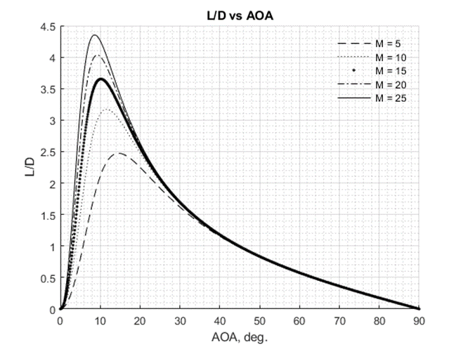
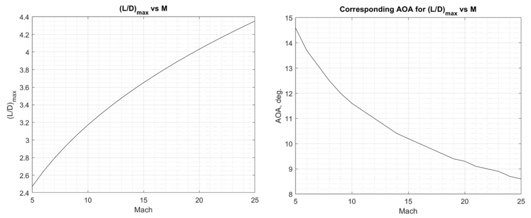
The organization of the weights is recorded by the author to ensure that there is consistency between the weight calculations and no double-counting.
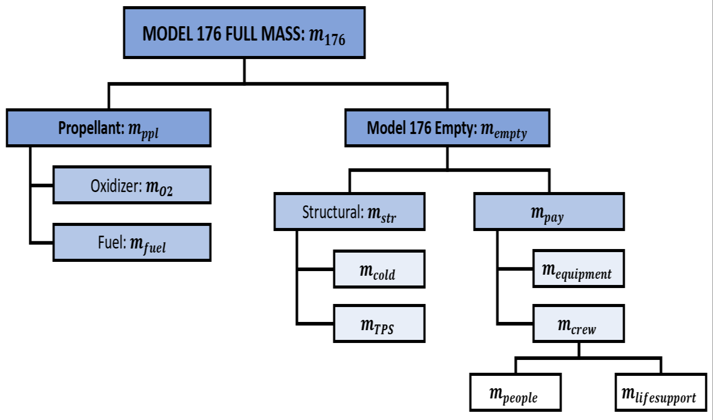
The weights shown above represent different methods for obtaining them. The payload weight is straightforwardly provided by the mission, where the crew needed and their associated life support system is easily computed in the mission chapter.
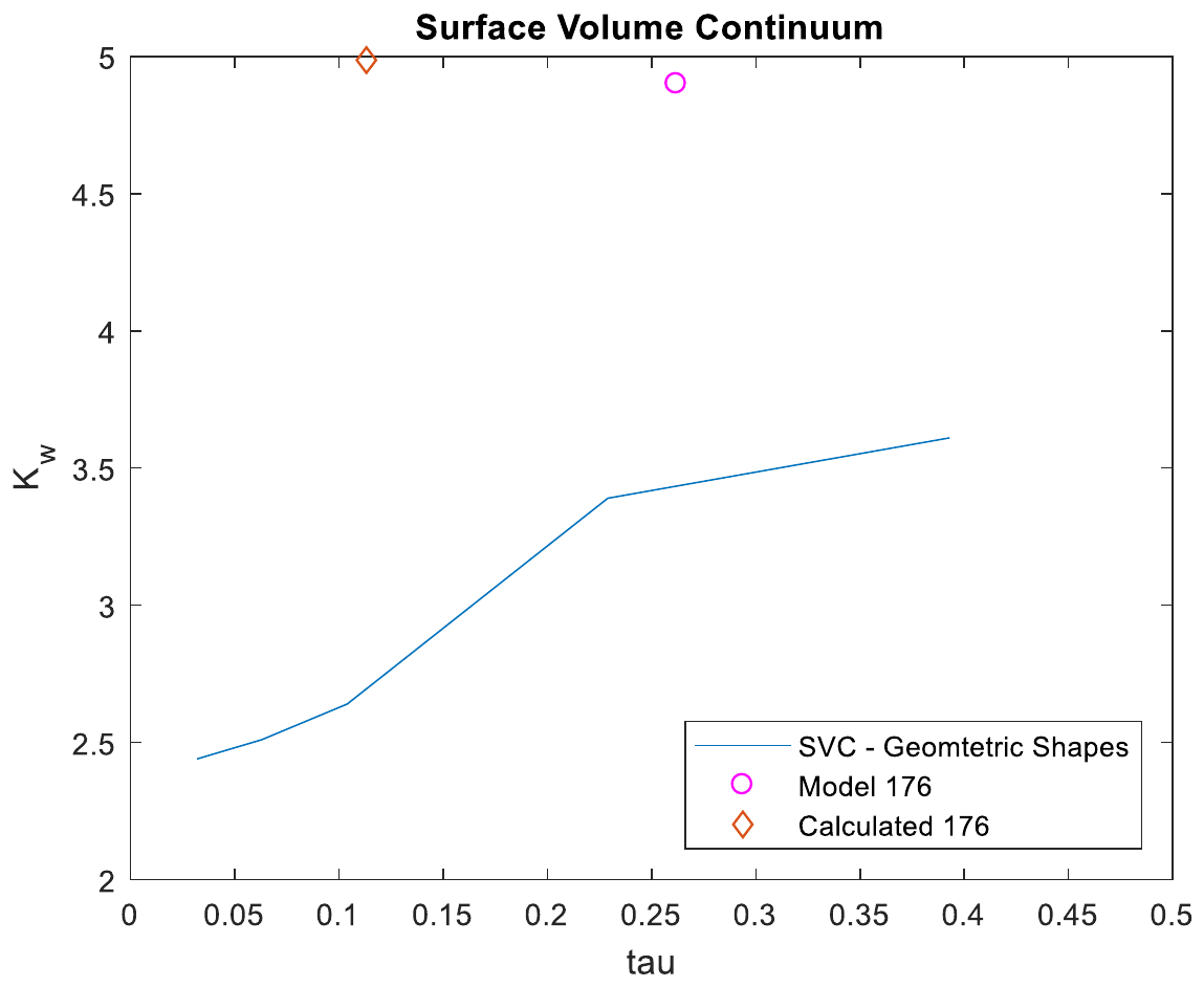
The CAD script is currently under development but will not be ready for the midterm as there is a huge difference between the methods used and the historical values, particularly when computing tau.
DSynthesis Script: Product Description
The Nassi-Schneiderman diagrams in the methodology chapter describe the process of analysis along with parallel processes, but the author believes it is also necessary to show code structure as it pertains to the various MATLAB subroutines developed by the individual disciplines. This more clearly displays the code hierarchy and the order they appear in the script. This is similarly shown in the table of contents within the script.
- Data Import
- Input Planet Geography
- Mission Trades
- Flight Domain Determination
- Hypersonic Analysis
- Determine Requirements
- Flight Profile and Disciplinary Analysis
- Finalize Layout
- Cost Evaluation
- Launch Analysis
- Vehicle Capability Determination
- Visualize
- Final Cost Evaluation
- Data Export
The flight profile and Disciplinary Analysis under “Hypersonic Analysis” is further broken down into the respective sub-team’s analysis by the following structure:
- Mission Requirements
- Flight Profile
- Flight Phase Bounds
- Select Critical Flight Phase
- Trajectory Analysis
- Critical Flight Phase
- Geometry Definition
- Propulsion
- Aerothermal
- Aerodynamics
- Heating
- Sizing
- Geometry Estimate
- Empty Weight Estimate
- Volume Required Estimate
- Weight Estimation
- Structures
- Stability and Control
- Stengel Method
- Clarke/Trimmer Method
- Wei Method (RCS Sizing)
- Geometry Redefinition
- Trajectory Analysis (Iterated)
- Comparison (Sizing)
- Cost Estimation
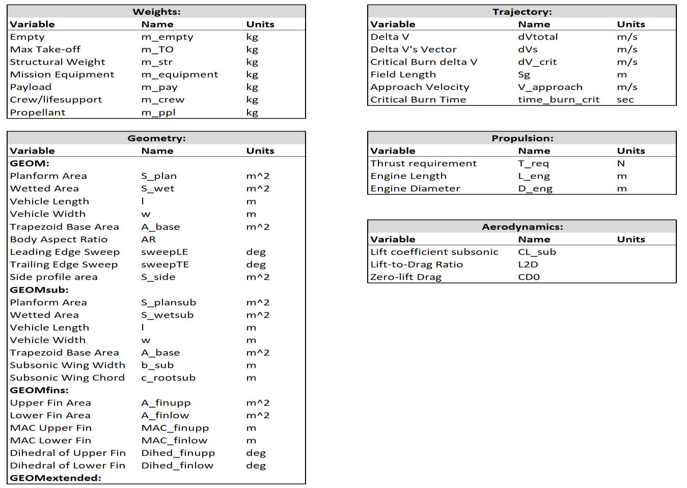
Below is a collection of variables which keep track of and standardize some common variables found in many disciplinary scripts.
Spotted an error, or want to reply? Email me: leonardo.pinero42 [at] gmail [dot] com