Design of Hypersonic Lifting Body Vehicle (Lead Chief Engineer’s Report) · Appendix

ADatabases

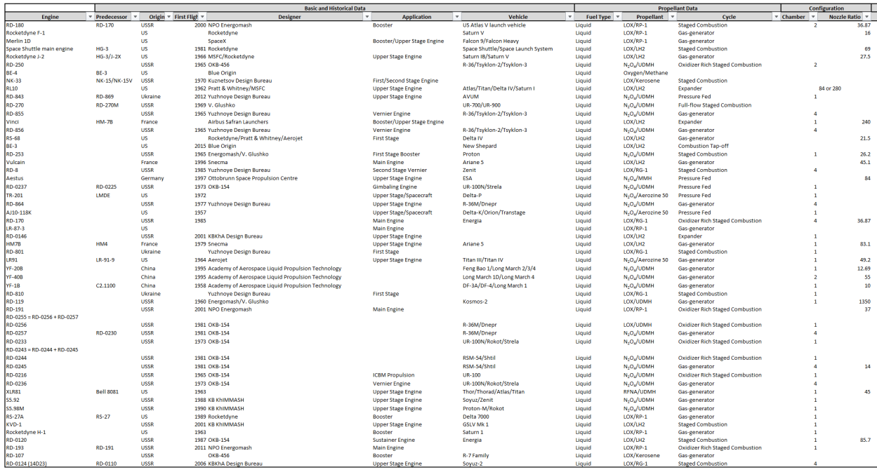
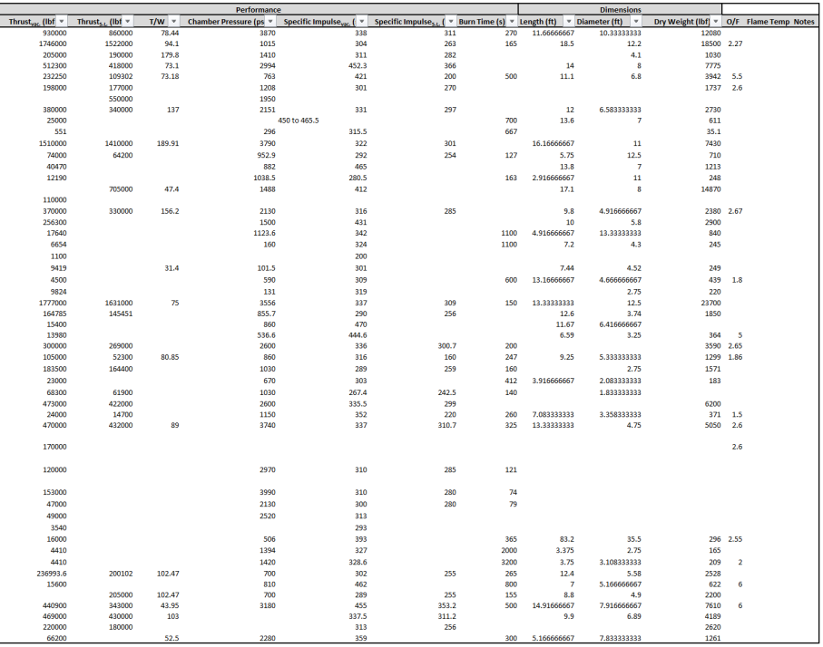
The following tables show the databases for the disciplines concerned. These are imported into the synthesis script to make judgements on the given data and plot trends. The propulsion database is shown below, which is a compendium of historical engine data.

BMATLAB Code

Below is the class script written by the author.

%%
%            ================================================
% ========================================================================
% ------------------------------------------------------------------------
% --------------   ASCENSION AEROSPACE DESIGN SCRIPT   -------------------
% ------------------------------------------------------------------------
% ========================================================================
%            ================================================

%{
WRITTEN BY:
Leonardo Pinero
%}

%{
CODE DESCRIPTION:
The following script will synthesize the two main sub-team scripts: one for
the Hypersonic Lifting Body Sub-team, and another for the Launch Sub-team.
The code takes mission and geographic parameters as inputs, and should
output a conceptual design of a combined vehicle reversed engineered from
the SpaceX launch vehicles and the McDonnel Model-176.
%}

%{
TABLE OF CONTENTS:
    Data Import
    Input Planet Geography
    Mission Trades
    Flight Domain Determination
    Hypersonic Analysis
        Determine L/D_req
        Flight Profile and Disciplinary Analysis
        Finalize Layout
        Cost Evaluation
    Launch Analysis
        ...
        ...
    Vehicle Capability Determination
    Visualize
    Final Cost Evaluation
%}



%%
% ==============================================
%                 DATA IMPORT
% ==============================================
%{
This section will preload all the outside variables. It can be commented
out to greatly save on computation time for further iterations.
%}

%

% User Interface:
Planet = xlsread('DesignMAE4351INPUT.xlsx', 'Planet', );
Mission = xlsread('DesignMAE4351INPUT.xlsx', 'Mission', );
Trade = xlsread('DesignMAE4351INPUT.xlsx', 'Trade', );

% Technical Database:
DATA = xlsread('DesignMAE4351DATA.xlsx', 'Eng', );


%

%%
% ==============================================
%             INPUT PLANET GEOGRAPHY
% ==============================================
% Written by: Leonardo Pinero
%{
inputs: Planet Data
outputs: Coordinates and flight path geometry
%}
Re = 6371000;  % planet radius [m]
g0 = 9.807;  % surface gravitational acceleration [m/s^2]

% ATMOSPHERIC PROPERTIES
% -------------------------------
T0 = 240; % average atmospheric temperature [K]

% composition:
N2  = 0.78;  % nitrogen
O2  = 0.21;  % oxygen
H2  = 0.00;  % hydrogen
CO2 = 0.00;  % carbon dioxide
Ar2 = 0.01;  % argon
MOL = (N2*28.04 + O2*32 + H2*2.02 + CO2*44.01 + Ar2*79.88)/1000; % atmospheric molecular weight

ATMOS_beta = MOL*g0/(8.314*T0);  % atmospheric scale height^(-1) [1/m]
ATMOS_scale = 1/ATMOS_beta;  % atmospheric scale height [m]

% SURFACE LOCATIONS
% -------------------------------
% Launch:
LAT_launch = 30;



%%
% ==============================================
%                MISSION TRADES
% ==============================================
% Written by: Leonardo Pinero
%{
inputs: mission requirements and user preferences
outputs: defined mission
%}


% TARGET FOR PARKING ORBITS:
% -------------------------------
% Target 1 (after launch):
LAT_park = 40;  % inclination of stable parking orbit [deg]
ALT_park = 200000;  % altitude of stable parking orbit [m]
VEL_park = sqrt(g0*Re^2/(Re + ALT_park));  % velocity of circular parking orbit [m/s]


% CROSS RANGE REQUIREMENT:
% -------------------------------
REQCrossRange = 1;  % cross range mission requirement
switch REQCrossRange % should be based on planetary radius
    case 1  % percent global coverage
%         cover = 0.95;  % percent coverage
%         L2Dreq = L2Dreq_globe(cover, Re);
        L2Dreq = 3.0;
    case 2  % continental US landing (Earth only)
        L2Dreq = 2.7;
    case 3  % Russian ladning (Earth only)
        L2Dreq = 1.8;
end



%%
% ==============================================
%          FLIGHT DOMAIN DETERMINATION
% ==============================================
% Written by: Leonardo Pinero
% TARGET COMBINED VEHICLE:
% -------------------------------
REQy = ALT_park;  % apogee of combined vehicle set to meet parking orbit [m]
REQi = LAT_park;  % inclination of combined vehicle set to that of parking orbit [deg]
REQvel = 7600;    % last velocity of combined vehicle [m/s]
if REQvel > VEL_park
    error('Launch overshoot. Consider decreasing REQvel requirements or increasing ALT_park.')
end
REQboost = VEL_park - REQvel;

ALT_stage = 100000;  % altitude of staging (should be launch performance output)

START = [ALT_stage, REQvel, ALT_park];  % [combined vehicle altitidue, combined vehicle velocity, desired parking orbit]



%%
% ==============================================
%            HYPERSONIC ANALYSIS
% ==============================================

% DETERMINE L/D_REQ
% -------------------------------
%{
inputs: Down Range requirement (DR)
outputs: Lateral Range (LR), L/D_req
%}
cover = 0.30;  % 30 percent circumferential coverage upon landing
L2Dreq_globe(cover, Re) % computation based on historical data


% FLIGHT PROFILE & DISC. ANALYSIS
% -------------------------------
%{
inputs:
outputs:
%}
iter = 0;
[W_176, Output Areas] = Hypersonic(Mission, DATAhyper, W_carried, START, iter);


% FINALIZE LAYOUT
% -------------------------------
%{
inputs:
outputs:
%}

% COST EVALUATION
% -------------------------------
%{
inputs:
outputs: cost estimation
%}



%%
% ==============================================
%              LAUNCH ANALYSIS
% ==============================================



%%
% ==============================================
%       VEHICLE CAPABILITY DETERMINATION
% ==============================================



%%
% ==============================================
%                 VISUALIZE
% ==============================================



%%
% ==============================================
%            FINAL COST ESTIMATION
% ==============================================

Below is hypersonic sub-team script written by the author, combining all of its disciplines and including their methods’ functions. This code interfaces with the launch sub-team.

function [W_176, Areas, STARTiter] = Hypersonic(Mission, DATAhyper, W_carried, START, iter)

% ========================================================================
% ----------------   HYPERSONIC STAGE DESIGN SCRIPT   --------------------
% ========================================================================

%{
WRITTEN BY:
Leonardo Pinero
%}

%{
CODE DESCRIPTION:
The following script will take two inputs: one database and a user
interface. The user interface contains the mission of the vehicle: a man-
rated hypersonic re-entry vehicle that can perform space operations, both
military and civilian. With user guidance, the script will converge on a
final conceptual design and give output plots and values.
%}

%{
TABLE OF CONTENTS:
    Mission Requirements
    Flight Profile
        Flight Phase Bounds
        Select Critical Flight Phase
    Trajectory Analysis
        Critical Flight Phase
    Geometry Definition
    Propulsion
    Aerothermal
        Aerodynamics
        Heating
    Sizing
        Geometry Estimate
        Empty Weight Estimate
        Volume Required Estimate
    Weight Estimation
    Structures
    Stability and Control
    Geometry Redefinition
    Trajectory Analysis (Iterated)
    Comparison (Sizing)
    Cost Estimation
%}



%%
% ==============================================
%             MISSION REQUIREMENTS
% ==============================================
%{
This section will process the Mission input and turn it into useful
variables for the disciplines.
%}

%{
Mission input breakdown:
[Inclination Change, Number of Crew Members, Time in Space, W_mission,
(L/D)_req]
%}

DeltLAT = Mission(1);
Ncrew = Mission(2);
Ndays = Mission(3);
L2Dreq = Mission(4);

VOL_pay = 1.247*Ncrew^0.136*Ndays^0.150;
m_crew = lifesupport(Ncrew, Ndays); % life support and crew estimation [kg]
m_pay = m_crew + m_equipment; % payload weight estimation



%%
% ==============================================
%               FLIGHT PROFILE
% ==============================================
%{
This section will actually develop a plotted flight profile which matches
the mission description. This is how the team will visualize the next
iteration.
%}




%%
% ==============================================
%            TRAJECTORY ANALYSIS
% ==============================================
%{
This section will take the flight profile and compute the velocity changes
needed to effect such a trajectory.
%}

% initial condition:
if iter == 0
    hi = START(1);
    Vi = START(2);
    h_des = START(3);
end

 % deltaV calculations:
dVs = Dvcalc(hi,Vi,h_des);

% Propulsion design-critical burn (thrust need)
dV_crit = 800;%max(abs(dVs));  % [m/s]
time_burn_crit = 240;  % [s]

% AERO INCLINATION TURN
% -------------------------------
[dV,V,hret] = AeroInc(W,S,CL,LD,h,sel);

%%
% ==============================================
%            GEOMETRY DEFINITION
% ==============================================
%{
This section will store information about the geometry and output it to
sizing and disciplines.
%}
[GEOM, GEOMsub, GEOMfins, GEOMextended GEOMall] = CADdefine(DATAhyper);

%{
GEOM: [Planform Area (S_plan), Wetted Area (S_wet), length of vehicle (l),
vehicle width (w), trapezoidal base (A_base), body aspect ratio (AR),
leading edge sweep (sweepLE), trailing edge sweep (sweepTE), Side profile
area (S_side) ]

GEOMsub: [Planform Area (S_plansub), Wetted Area (S_wetsub), length of
vehicle (l), vehicle width (w), trapezoidal base (A_base), subsonic wing
width (b_sub), switchblade wing chord (c_rootsub) ]

GEOMfins: [ upper fin area (A_finupp), lower fin area (A_finlow), MAC upper
fin (MAC_finupp), MAC lower fin (MAC_finlow), dihedral of the upper fin
(Dihed_finupp), dihedral of the lower fin (Dihed_finlow) ]

GEOMextended: [ Weight balance inputs ]

GEOMall: [GEOM; GEOMsub; GEOMfins; GEOMextended] matrix of geometry
(preallocate with a zero matrix of a large enough size to avoid matrix
dimensional issues)
%}


l = GEOM(1);
w = GEOM(2);
S_plan = GEOM(3);
S_wet =

% Output to rocket team:
Areas = [S_side, S_plan];



%%
% ==============================================
%                 PROPULSION
% ==============================================

% SIZING ENGINE FOR THRUST REQ
% -------------------------------
T_req = W_carried*dV_crit/time_burn_crit;  % critical burn requirement from traj
[T2W_eng, D_eng, L_eng, m_eng] = PropulsionSizingFunction(T_req);
% _eng subscript relates to engine
VOL_eng = pi*(D_eng/2)^2*(0.5*L_eng);  % engine volume assumed to be cylindrical, considers volume INSIDE ship

% SIZING TANKS FOR DELTA V REQ
% -------------------------------



%%
% ==============================================
%                AEROTHERMAL
% ==============================================

% SUBSONIC AERODYNAMICS
% -------------------------------
[CLsub, CDsub, L2Dsub, L2D_maxsub] = subsonic(WL_sub, l, A_b, b_sub, S_wetsub, S_refsub);

% HYPERSONIC AERODYNAMICS
% -------------------------------
[CL, CD, L2D, L2D_max] = hyper(l, A_b, S_wet, Sref, W_empty);

% NEUTRAL POINT
% -------------------------------
[NPsub, NP] = NPcalc(GEOM);

% THERMAL LOADS
% -------------------------------
Thermmap(W,S,CL,R0,Tmin,Tmax,Tint,points)  % Written by Chris Miller


%%
% ==============================================
%                  SIZING
% ==============================================



%%
% ==============================================
%               WEIGHT ESTIMATION
% ==============================================
% Build massINPUT
massINPUT = [ ];

[m_str, m_component] = massEstimate(massINPUT);
m_empty = m_str + m_ppl + m_pay


%%
% ==============================================
%                STRUCTURES
% ==============================================
%{
Takes aerothermal loads and outputs required structural weight and
geometry.
%}



%%
% ==============================================
%            STABILITY AND CONTROL
% ==============================================

% STENGEL METHOD
% -------------------------------
StaCon_Input = [l, w, S_plan, A_base, VOL, croot_sub, b, CG_empty, yMAC, MAC, NPsub, NP, CD0sub, sweepLE, sweepTE, AR, S_finupp, S_finlow, MAC_finupp, MAC_finlow, Dihed_finupp, Dihed_finlow];
%{
StaCon_Input (25 GEOM components in index order):

body length, maximum body width, reference area, base area, volume,
wing root chord, wing span, CG location from tip, yMAC, MAC, NP subsonic
(from tip), NP supersonic (from tip), parasitic drag, LE sweep, TE sweep,
AR of the body, upper fin area, lower fin area, MAC upper fin, MAC lower
fin, dihedral of the upper fin, dihedral of the lower fin.
%}

% Stengel Method:
[SC1] = StaCon_Function(StaCon_Input);
% SC1 Guide 1-9: M, Cma, CYb, Cnb, Clb, Cmde, CYdr, Cndr, Clda
figure
hold on
plot(SC1(1,:),SC1(2,:), 'k', 'LineWidth', 2)
title('C_{M\alpha} vs. Mach')
xlabel('Mach Number')
ylabel('C_{M\alpha}')
grid on
grid minor
hold off

% CLARKE/TRIMMER METHOD
% -------------------------------


% WEI METHOD (RCS SIZING)
% -------------------------------



%%
% ==============================================
%             GEOMETRY REDEFINITION
% ==============================================

% GEOMETRY SIZING CHECK
% -------------------------------
%{
This function will act as the CAD check and is a MATLAB stand-in for the
discipline’s tools: SOLIDWORS and OpenVSP.
%}
GeomSizing(S_plan, S_wet, GEOM, VOL)  % void function



%%
% ==============================================
%             COMPARISON (SIZING)
% ==============================================



%%
% ==============================================
%          TRAJECTORY ANALYSIS (ITERATED)
% ==============================================

% SUBSONIC ANALYSIS
% -------------------------------
[range_sub, V_approach, Sg, gamma_approach] = subsonic_perf(L2D_maxsub,CLsub,CL_maxsub,S_plansub,W_empty,hsub);

% Sg = field length



%%
% ==============================================
%             COMPARISON (BUDGET)
% ==============================================



%%
% ==============================================
%              COST ESTIMATION
% ==============================================



end

Below is the author’s script to relate cross-range capability to required lift-to-drag.

function L2Dreq_globe(cover, Re)
% Written by: Leonardo Pinero

L2D = 0:0.025:3;
LR = 0.539957*(1.667 + 68.016.*L2D + 706.67.*L2D.^2 - 91.111.*L2D.^3);  % [km]
DR = 4866.6 + 4.70417.*LR;  % [km]
circum = zeros(length(L2D), 1) + (Re/1000)*2*pi;
circum_half = circum./2;

reqDR = cover*circum;

hold on
plot(L2D, LR, 'k--')
plot(L2D, DR, 'k')
plot(L2D, circum_half, 'k', 'LineWidth', 2)
plot(L2D, reqDR, 'r', 'LineWidth', 3)
legend('Lateral Range', 'Down Range', 'Half of Earth''s Circumference', 'Required Range', 'Location', 'Best')
title('Range vs. L/D (30% Circumferential Coverage Requirement)')
xlabel('Lift to Drag Ratio')
ylabel('Range [km]')
grid on
grid minor
hold off

end

Below are the trajectory functions from performance, used to derive the vehicle’s disciplinary requirements from the mission profile and Earth’s geography [15].

Inclination change:

function  [dV,V,hret] = AeroInc(W,S,CL,LD,h,sel)
%AeroInc_a
%Christopher Miller
%7/2/18

%inputs
W = W * 2.2; %vehicle weight, lb
S = S* 10.763; %wing reference area, ft^2
%CL = .2; %lift coefficient
%LD = 3; %lift-drag ratio
h = h*3.28; %ft
WSCL = W/(S*CL);
WCDA = 1000;

%constants
R0 = 6371000 * 3.28; %ft
B = 1/24000; %1/ft
u0 = 25940; %ft/s
d0 = .07648; %sea level air density, lbm/ft^3

dVi = Dvcalc(h/3.28,0,34.4*6076/3.28);
dV = dVi(1);

 %insertion
ri = R0+h;
if sel == 0
    %hohmann
    uiu0 = sqrt((2*1.01)/((ri/R0)*(1.01+ri/R0)));
    gammar = 0;
    uru0 = sqrt(2)/1.01*sqrt((1.01*(ri/R0)/(1.01+ri/R0)));
    ui = uiu0*u0; %iniital velocity
    ur = uru0*u0; %reentry velocity
end
if sel == 1
    %ballistic
    uiu0 = sqrt(1.01)*R0/ri;
    gammar = atan(1.01*R0/ri - 1);
    uru0 = 1/sqrt(1.01)*cos(gammar);
    ui = uiu0*u0;
    ur = uru0*u0;
end

%pullout
if sel == 1
    u0u = ((ri/R0)*(ui/u0)*cos(0))/(((63708.8*3.28 + R0)/R0)*cos(gammar))^-1;
    u = ur/((exp(gammar*(1/LD)*(1 + (u0u^2-1)/(B*R0*(1-cos(gammar)))))));
    hp = -1/B*log((2*WSCL*B/d0)*(1-cos(gammar)+1/(B*R0)*(u0u^2 - 1)));
    uru = exp((R0*d0*(deg2rad(2))*exp(-B*hp))/(2*WCDA*cos(deg2rad(2))*(u0u^2-1)));
end

%glide
lambda = pi/3; %60 deg. minor circle
pos = pi/2.88703; %position coordinate for 30 deg plane change
i = asin(sin(pos)*cos(lambda)*sqrt(1 + (1-cos(pos))/(1+cos(pos))*sin(lambda)^2));
rad2deg(i)
xi = ur/u0;
Fxi = 1 - xi^2/sin(lambda)^2 - 1/sin(lambda)*sqrt(xi^4/sin(lambda)^2 - 2*xi^2 + 1);
Fx = exp(log(abs(Fxi))-2*pos/LD);
x = sin(lambda)*sqrt(-Fx^2 + 2*Fx + csc(lambda)^2 - 1)/(sqrt(2)*sqrt(Fx));
dV(2) = (u0-x*u0)/3.28;
dVi = Dvcalc(34.4*6076/3.28,0,h/3.28);
dV(3) = dVi(1);
dV(4) = dVi(2);
V = [ur/3.28 x*u0/3.28];
hret = 34.4*6076/3.28;

end

Delta V calculations:

function dVs = Dvcalc(h,Vin,h_des)
% Written by: Christopher Miller

%input
%h = 200000;
%V = [7784 0];
Re = 6371000; %km
me = 5.972e24; %kg
G = 6.67408e-11;
mu = G*me;
a_des = h_des + Re;
if Vin == 0
    Vin = sqrt(mu/(h+Re));
    V = [Vin 0];
else
    V = Vin;
end

R = [0; Re+h];
r = norm(R);
v = norm(V);
e = ((v.^2-mu/r)*R - (dot(R,V)*V))/mu;
es = norm(e);
a = 1/(2/r-v^2/mu);
E_1 = -mu/(2*a);
apo = a*(1+es^2);
peri = a*(1-es^2);
va_1 = sqrt(2*(E_1+mu/apo));

E_2 = -mu/(2*((a_des+peri)/2));

vp_2 = sqrt(2*(E_2+mu/apo));
dVs(1) =  vp_2-va_1;

vcirc = sqrt(mu/a_des);
va_2 = sqrt(2*(E_2+mu/a_des));
dVs(2) = vcirc-va_2;

end

Subsonic performance:

function [range_sub,Vapp,Sgland,gammaa]  = subsonic_perf(LDmax,CL,CLmax,S,W,hi)
% Written by: Christopher Miller

g = 9.81;

gammaa = atan(LDmax^-1);
range_sub = hi*cos(gammaa)/sin(gammaa);

rho = atmos(0:10:10000,'Units','SI');

V = sqrt(W./(.5.*rho.*S*CL*(cos(gammaa)+LDmax^-1*sin(gammaa))));

plot(V,0:10:10000,'k')
grid on
grid minor
xlabel('Velocity, m/s')
ylabel('Altitude, m')
title('Subsonic glide velocity')

fprintf('Subsonic glide range: %0.0f m\n',range_sub)
n = 1.5;
WSland = W/S;
Vsland = sqrt(WSland * 2/(rho(1)* CLmax));
Vapp = Vsland * 1.2;
Vtd = Vsland * 1.1;
gammaapp = gammaa;
Rapp = mean(Vapp+Vtd).^2/(g*(n-1));
hflare = Rapp*(1-cos(gammaapp));
Ktapp = -.3;
Kaapp = rho(1)/(2*(WSland))*(.3*.05-.0095-.0535*.05^2);
Sgland = 1/(2*g*Kaapp)*log((Ktapp)/(Ktapp+Kaapp*Vtd^2)) + 3*Vtd;
fprintf('Approach angle: %0.0f degrees\n',gammaapp*180/pi)
fprintf('Approach speed: %0.2f m/s, \n',Vsland)
fprintf('Landing distance assuming 3 second ground roll after touchdown:
%0.0f m\n', Sgland)

end

Thermal mapping:

function stuff = Thermmap(W,S,CL,R0,Tmin,Tmax,Tint,points)
% Written by: Christopher Miller

WSCL = W/(S*CL);%input('Specify W/(S*CL): ');
% points = 100;%input('Specify number of data points: ');
% R0 = .1;%input('Specify LE radius (m): ');
% Tmin = 300;%input('Specify desired min temp (K): ');
% Tmax = 1900;%input('Specify desired max temp (K): ');
% Tint = 200;%input('Specify desired temp interval: ');

T = [Tmin:Tint:Tmax];
Re = 6371000;
g = 9.81;

H = [0:100000/(points-1):100000];
rho = atmos(H,'units','SI');

V = (1./(g*(Re+H))+ rho./(2*WSCL)).^(-1/2);
V2 = (1./(g*(Re+H))+ rho./(2*600)).^(-1/2);

lim = size(T);
i = 1;
Vt = zeros(lim(2),points);
while i <= lim(2)
   Vt(i,:) = ((T(i).^4*5.67e-8*.8)./(1.83e-4*sqrt(rho./R0))).^(1/3);
    i = i + 1;
end
hold on
grid on
grid minor
for i = 1:lim(2)
    if mod(i,2) == 1
        plot(Vt(i,:),H,'k')
    end
    if mod(i,2) == 0
        plot(Vt(i,:),H,'--k')
    end
end
plot(V,H,'r')
plot(V2,H,'--r')
axis([0 10000 50000 100000])
xlabel('Velocity,m/s')
ylabel('Altitude,m')
entries = cell(length(T),1);
for i = 1:length(T)
    entries{i} = [num2str(T(i)) ' K'];
end
entries{length(T)+1} = ['Re-entry profile, W/SCL = ' num2str(WSCL)];
entries{length(T)+2} = ['Re-entry profile, W/SCL = 600'];
title('Thermal Map, temp increases moving right')
legend(entries,'Location','SE')
end

Trajectory code:

%Performance and Trajectory - code link
%Christopher Miller
%7/7/2018

clear
clc
close all

%Test Case Variables
LDmaxsub = 6;
CLsub = .2;
CLmaxsub = .5;
Ssub = 15;
Wsub = 10000;
hsub = 10000;
hi = 70000;
Vi = [6800 100];
h_des = 200000;
W = 12000;
S = 60;
LDmax = 3;
CL = .15;
h_circ = 200000;
sel = 0;
R0 = .1;
Tmin = 700;
Tmax = 1900;
Tstep = 200;
points = 100;

%Subsonic - range calculation, landing speed, field length
%Inputs: L/Dmax, CL for L/Dmax, foldout wing area, vehicle weight, initial
%height
%Outputs: range during subsonic flight,landing field length, approach
%velocity, approach flight path angle, plot of optimum glide speed vs
altitude

[Range, Vapp, Sg, gammaa] = subsonic_perf(LDmaxsub,CLsub,CLmaxsub,Ssub,Wsub,hsub);

%Dvcalc - calculates dV's required for Hohmann transfers between orbits
%Inputs: vehicle altitude, current velocity, desired circular orbit
%altitude
%Outputs: a vector with 2 values for the impulses required (at
%initial/transfer orbit apogees) to insert the vehicle into the desired
%circular orbit

dVi = Dvcalc(hi,Vi,h_des);

%AeroInc - calculates the enviroment and delta-V requirement for the
%orbital plane change maneuver (assumes 30deg)
%Inputs: Vehicle weight, hypersonic reference area, Cl for l/dmax,
%l/dmax, initial orbit altitude (must be circular), selector for hohmann or
%ballistic reentry (suggest hohmann for now ballistic is wonky)
%Outputs: four required dV's, max/min atmosphere speed, altitude for those
%speeds (constant altitude glide phase)

[dVs, Vspec, h_t] = AeroInc(W,S,CL,LDmax,h_circ,sel);

%Thermmap - determines re-entry trajectory and thermal map for said
%trajectory
%Inputs: W,S,CL, nose radius, Temperature ranges as three variables: Tmin, Tmax, Tstep; # data points (typically 100)
%Outputs: Plot of thermal map, currently outputs no variables

hold on
figure
Thermmap(W,S,CL,R0,Tmin,Tmax,Tstep,points);

Below is CAD’s life support function which aids in defining payload parameters from the mission description. [36] This is based on the realities and human studies of living in space.

function [W_tot] = lifesupport(Ncrew, Ndays)
% Written by Jared Arizpe
% Recon
% This will calculate crew/passenger payload for 'x' days
W_pass = 92; %Weight of 6' male in kg
W_crew = (Ncrew*W_pass); %total weight of crew
O2 = 0.9; %O2 usage/man day in kg.
H2O = 9.1; %H2O usage/man day in kg. Includes drinking and wash
Food = 0.6; %Food usage/man day in kg.
W_lifesupport = (O2+H2O+Food)*Ncrew*Ndays;

W_tot = W_crew + W_lifesupport;
end

Descent script made to replicate literature search plots and use as a tool for testing out different design parameters.

%{
===========================================================================
========================   PLOTTING DESCENT   =============================
===========================================================================
%}
close all



%%
% CONSTANT SETTINGS
% ---------------------------------
Re = 6371000; % earth's radius [m]
g0 = 9.807;  % gravitational acceleration at sea level [m/s^2]
K = g0*Re^2;  % gravitational constant



%%
% INITIALIZE
% ---------------------------------
% Kinematics:
% gamma =  % entry angle
% Vorb =  % orbital speed

% Design:
% CL =  % coefficient of lift
% S =  % planform area
% CD =  % coefficient of drag

% Altitudes examined:
% h1 = 1000*(0:.1:30);  % low altitudes high resolution [m]
% h2 = 1000*(30:2:150);  % high altitudes low resolution [m]
% h = [h1, h2(2:end)];  % combine into one vector
% clear h1 h2
h = 1000*(40:2:150);  % altitude observed: 40 km - 150 km

% Pre-load atmos properties
[~,~,~,rho] = atmoscoesa(h, 'None');  % 1976 extended atmosphere



%%
% TRAJECTORY PLOTTER
% ---------------------------------
figure
%{
WSCL1 = 1:20;
WSCL2 = 30:10:140;
WSCL3 = 150:50:700;
WSCL4 = 750:250:2000;
%}

% WSCL = [WSCL1 WSCL2 WSCL3 WSCL4];
WSCL = [30, 100, 1000];
Vc = sqrt(K./(Re + h));

hold on
title('Descent Trajectories for Different Values of $\frac{W}{SC_L}$', 'Interpreter', 'Latex')
xlabel('Velocity [km/s]', 'Interpreter', 'Latex')
ylabel('Altitude [km]', 'Interpreter', 'Latex')
grid on
grid minor
for i = 1:length(WSCL)
    V = (1./Vc.^2 + rho./(2.*WSCL(i))).^(-1/2);
    if mod(i,3) == 0
        plot(V./1000,h./1000, 'k')  % converting from [m] to [km]
    elseif mod(i,3) == 1
        plot(V./1000,h./1000, 'k:', 'LineWidth', 2)  % converting from [m] to [km]
    else
        plot(V./1000,h./1000, 'k--')  % converting from [m] to [km]
    end
end

% legend entries:
WSCLentries = cell(length(WSCL),1);
for i = 1:length(WSCL)
    WSCLentries{i} = ['W/(SC_L) = ' num2str(WSCL(i))];
end
hold off
legend(WSCLentries, 'Location', 'Best')

Below is the analysis code used for mission trade studies and associated sub-routines (continuously modified to make different plots).

% NYLAND PLOTTER
% ---------------------------
% written by: Leonardo Pinero
% date: 31 July 2018
% close all

% Inputs:
PLANET = [1.2, 8500, 6371000, 9.807]; %Mars: [0.02, 11100, 3396000, 3.71];
DV = 123:200:20000;
L2D = 3;
K = PLANET(4)*PLANET(3)^2;
rh = PLANET(3) - PLANET(2)*log(0.000676/PLANET(1));  % density to turn: 0.000676 kg/m^3


% PLOT DELTA I vs DELTA V
DI = zeros(length(L2D), length(DV));  % preallocate
hold on
for i = 1:length(L2D)
    for j = 1:length(DV)
    DI(i,j) = nyland(DV(j), L2D(i), PLANET);
    end
    %{
    % USE IF NEED TO SEE REQ'S FOR HIGHER DELTA I ANGLES
    DIbig = unwrap(3*DI, pi);
    DI = DIbig./3;
    %}
    if mod(i,4) == 0
        plot(DV, rad2deg(DI(i,:)), 'k', 'LineWidth', 1.5)
    elseif mod(i,4) == 1
        plot(DV, rad2deg(DI(i,:)), 'b--', 'LineWidth', 1.5)
    elseif mod(i,4) == 2
        plot(DV, rad2deg(DI(i,:)), 'b--')
    else
        plot(DV, rad2deg(DI(i,:)), 'k--', 'LineWidth', 1.5)
    end
end
DVprop = 0:200:20000;
DIprop = zeros(1, length(DVprop));  % preallocate
for i = 1:length(DVprop)
    DIprop(i) = PropIncline(DVprop(i), PLANET);
end
plot(DVprop, rad2deg(DIprop), 'b', 'LineWidth', 2)
ufinish = sqrt(K/rh);
xlim([0, ufinish])
DeltaIreq = zeros(length(DV),1) + 30;
plot(DV, DeltaIreq, 'k:', 'LineWidth', 3)
title('$\Delta$i per $\Delta$V with $\frac{L}{D}$ = 3 on Earth and Mars', 'Interpreter', 'Latex')
xlabel('$\Delta V_{required}  [\frac{m}{s}]$', 'Interpreter', 'Latex')
ylabel('$\Delta$i [deg]', 'Interpreter', 'Latex')
grid on
grid minor

% legend entries:
L2Dentries = cell(length(L2D),1);
for i = 1:length(L2D)
    L2Dentries{i} = ['Earth L/D = ' num2str(L2D(i))];
end
L2Dentries{length(L2D) + 1} = 'Earth Propulsive Maneuver';
L2Dentries{length(L2D) + 2} = 'Mission';
hold off
legend(L2Dentries, 'Location', 'Best')

Nyland analysis sub-routine shown below.

function [DeltaI, phi, dv2] = nyland(DeltaV, L2Dturn, PLANET)

%{
% test case:
PLANET = [7317, 6371000, 9.81];  % scale, radius, surface
gravity
DeltaV = 2100;
L2Dturn = 2;
%}

% DATA/SETTINGS:
% ---------------------------------
% break down planet rack:
rho_sea = PLANET(1);
atmos_scale = PLANET(2);  % atmospheric scale height
Re = PLANET(3);  % planet radius
g0 = PLANET(4);  % surface gravity

% deal with negative L2D's
L2Dturn = abs(L2Dturn);

% environmental constants
K = g0*Re^2;
u0 = sqrt(K/Re);  % earth skimming velocity

gamma = deg2rad(45);  % minor circle cone angle



% METHODS:
% ref: Nyland, Rand Corporation
% ---------------------------------
% find delta V required to descend and re-circularize:
ALTturn = -atmos_scale*log(0.000676/rho_sea);  % density to turn: 0.000676 kg/m^3

ri = Re + 200000;  % initial sattelite height
rh = Re + ALTturn;

% deltaV required to burn to and from this altitude
ui = sqrt(K/ri);  % initial circular velocity at ri
uapo = sqrt((2*K*rh)/(ri*(ri + rh)));  % descent ellipse
uperi = sqrt((2*K*ri)/(rh*(ri + rh)));  % descent ellipse
ufinish = sqrt(K/rh); % velocity at end of turn (descent ellipse now circularized)

dv1 = ui - uapo;  % dv1 is used twice for mission (we need to return home!)
dv4 = dv1;  % recircularize
dv3 = uperi - ufinish;  % dv req to get from unfinish back up to orbit
dvatmos = DeltaV - (2*dv1 + dv4);  % deltaV available after orbit ops
dv2 = dvatmos - dv3;

if dv2 < 0
    if dv3 < 0
        DeltaI = 0;
    else
        while dv2 < 0
            ufinish = (ufinish + uperi)/2; % cut the turn short, not enough fuel!

            % run dv calcs again until we can get some dv2
            ui = sqrt(K/ri);
            uapo = sqrt((2*K*rh)/(ri*(ri + rh)));
            uperi = sqrt((2*K*ri)/(rh*(ri + rh)));
            dv1 = ui - uapo;
            dv4 = dv1;
            dv3 = uperi - ufinish;
            dvatmos = DeltaV - (2*dv1 + dv4);
            dv2 = dvatmos - dv3;

            u = ufinish - dv2;
            phi = 0.5*L2Dturn*(log(rangefunc(uperi, u0, gamma)) - log(rangefunc(u, u0, gamma)));
            DeltaI = asin(sin(phi)*sin(gamma)*sqrt(1 + (1 - cos(phi))/(1 + cos(phi))*(sin(gamma))^2));

        end
    end

else
    u = ufinish - dv2;
    phi = 0.5*L2Dturn*(log(rangefunc(uperi, u0, gamma)) - log(rangefunc(u, u0, gamma)));
    DeltaI = asin(sin(phi)*sin(gamma)*sqrt(1 + (1 - cos(phi))/(1 + cos(phi))*(sin(gamma))^2));
end


% corrections for high performance
% NOT NEEDED (removed):
%{
if (deg2rad(90) - DeltaI) < -87.5
    DeltaI = real(DeltaI + deg2rad(180));  % maxed out performance for gamma = 45 deg
elseif isreal(DeltaI) == 0
    DeltaI = real(deg2rad(90) - DeltaI);  % maxed out
performance for gamma = 45 deg
end
%}

DeltaI = abs(DeltaI);

% correct for high performance:
%{
[DeltaITEST1, ~] = nylandTEST(0.95*DeltaV, L2Dturn, PLANET);
if DeltaITEST1 > DeltaI % passed the north pole, increased dv incorrectly lowers DeltaI
    DeltaI = 2*nylandTEST(ufinish, L2Dturn, PLANET) - DeltaI;  % restate the true performance
end
%}
    function [F] = rangefunc(u, u0, gamma)
        x = u/u0;
        F = 1 - x^2/(sin(gamma))^2 - 1/sin(gamma)*sqrt(x^4/sin(gamma)^2 - 2*x^2 + 1);
    end


end

Spotted an error, or want to reply? Email me: leonardo.pinero42 [at] gmail [dot] com